ch8_conditional_manatees
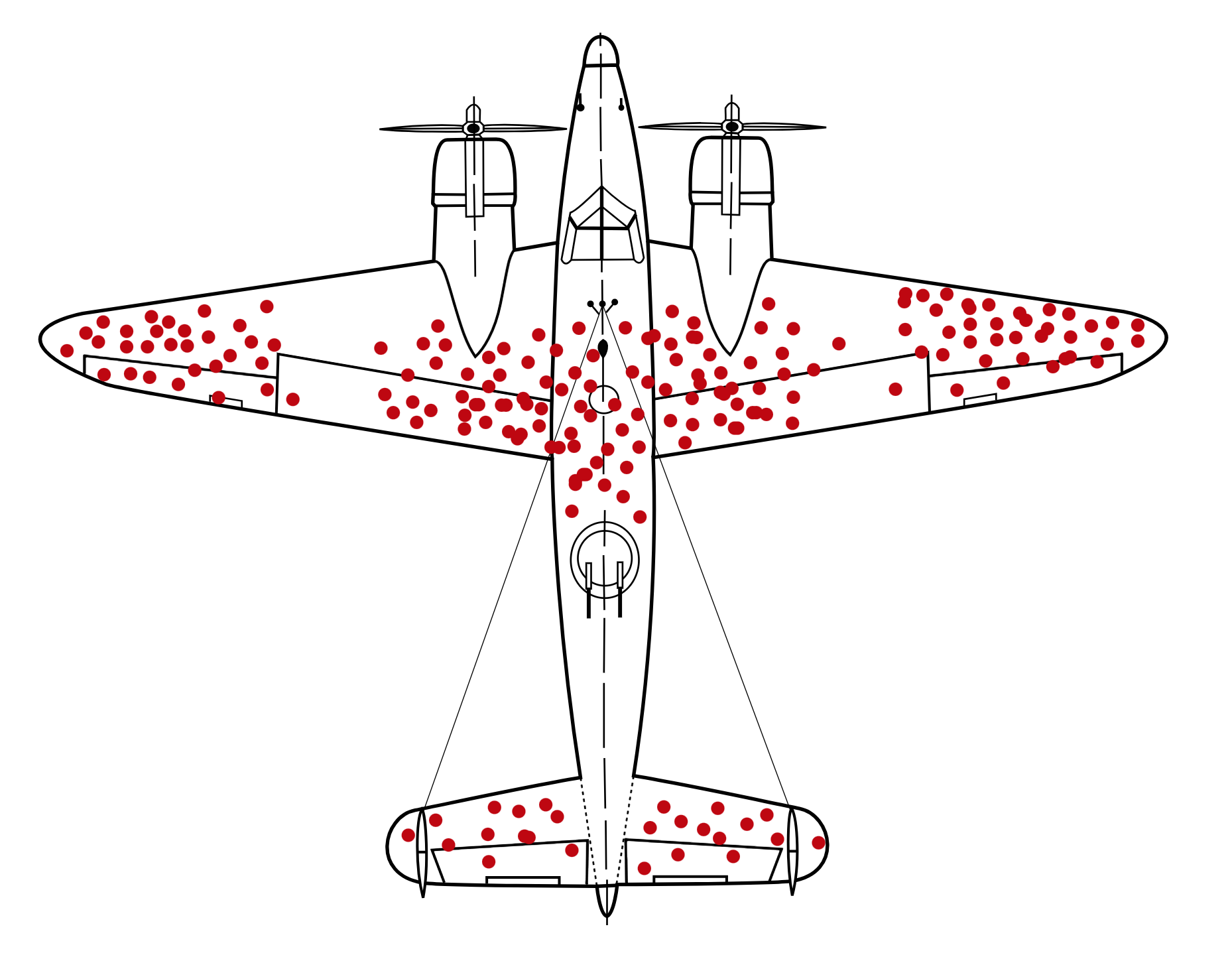
The Armstrong Whitworth A.W.38 Whitley was a frontline Royal Air Force bomber. During the second World War, the A.W.38 carried bombs and pamphlets into German territory. The A.W.38 has fierce natural enemies: artillery and interceptor fire. Many planes never returned from their missions. And those that survived had the scars to prove it. Most observers intuit that helping bombers means reducing the kind of damage we see on them, perhaps by adding armor to the parts of the plane that show the most damage.
Up-armoring the damaged portions of returning bombers did little good. Instead, improving the A.W.38 bomber meant armoring the undamaged sections. The evidence from surviving bombers is misleading, because it is conditional on survival. Bombers that returned home conspicuously lacked damage to the cockpit and engines. They got lucky. Bombers that never returned home were less so. To get the right answer, in either context, we have to realize that the kind of damage seen is conditional on survival.
Conditioning is one of the most important principles of statistical inference. Data, like the bomber damage, are conditional on how they get into our sample. Posterior distributions are conditional on the data. All model-based inference is conditional on the model. Every inference is conditional on something, whether we notice it or not.
Simple linear models frequently fail to provide enough conditioning, however. Every model so far in this book has assumed that each predictor has an independent association with the mean of the outcome. What if we want to allow the association to be conditional? For example, in the primate milk data from the previous chapters, suppose the relationship between milk energy and brain size varies by taxonomic group (ape, monkey, prosimian). This is the same as suggesting that the influence of brain size on milk energy is conditional on taxonomic group. The linear models of previous chapters cannot address this question.
To model deeper conditionality—where the importance of one predictor depends upon another predictor—we need interaction (also known as moderation). Interaction is a kind of conditioning, a way of allowing parameters (really their posterior distributions) to be conditional on further aspects of the data.
More generally, interactions are central to most statistical models beyond the cozy world of Gaussian outcomes and linear models of the mean. In generalized linear models (GLMs), even when one does not explicitly define variables as interacting, they will always interact to some degree. Multilevel models induce similar effects. Common sorts of multilevel models are essentially massive interaction models, in which estimates (intercepts and slopes) are conditional on clusters (person, genus, village, city, galaxy) in the data. Multilevel interaction effects are complex. They’re not just allowing the impact of a predictor variable to change depending upon some other variable, but they are also estimat- ing aspects of the distribution of those changes. This may sound like genius, or madness, or both. Regardless, you can’t have the power of multilevel modeling without it.
Discrete ~Continuous Interactions
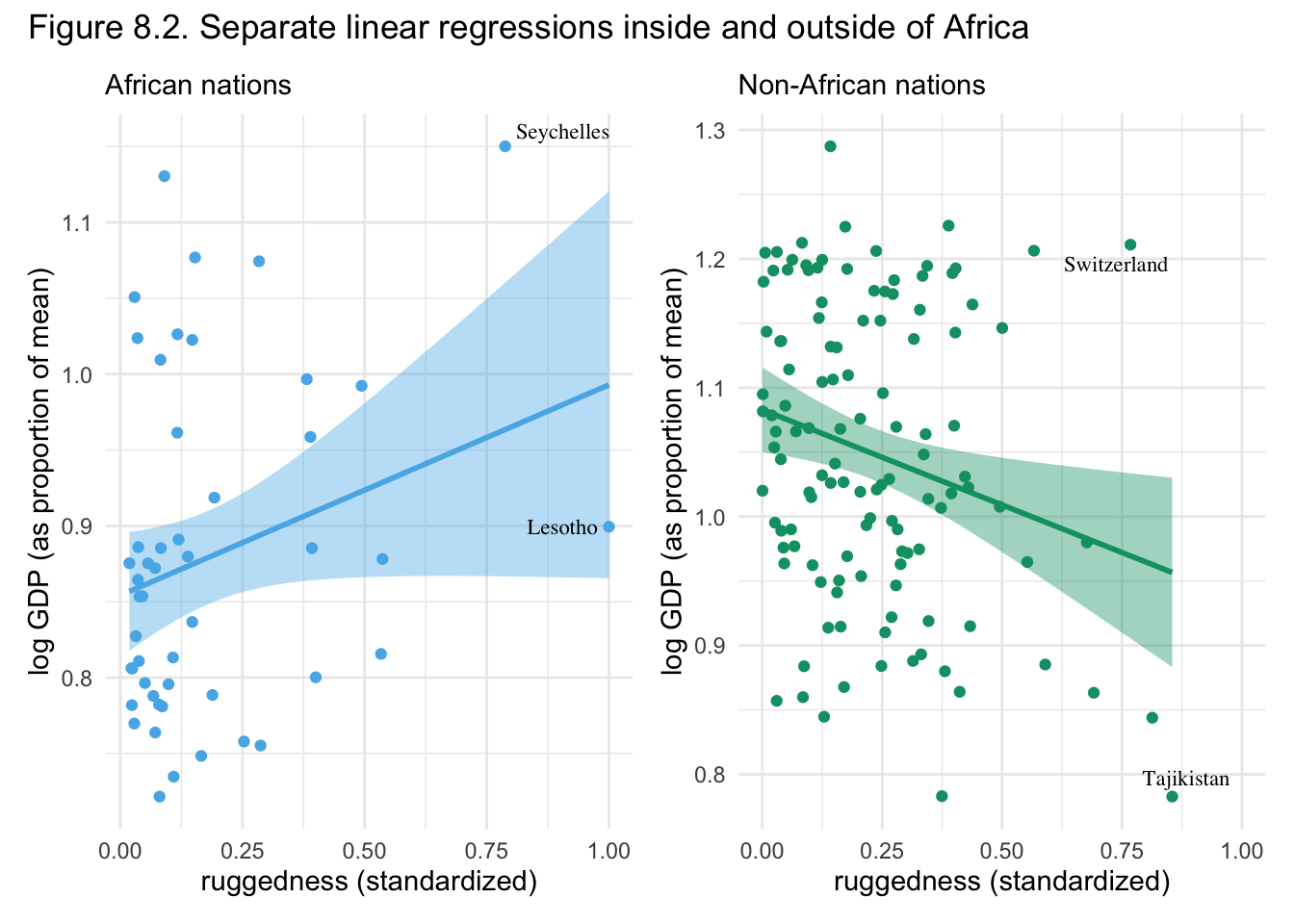
Ruggedness vs GDP in Africa 🌍
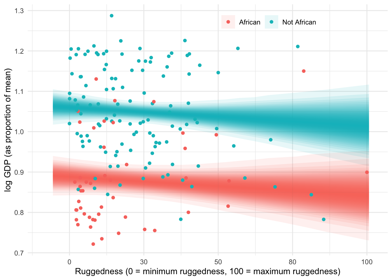
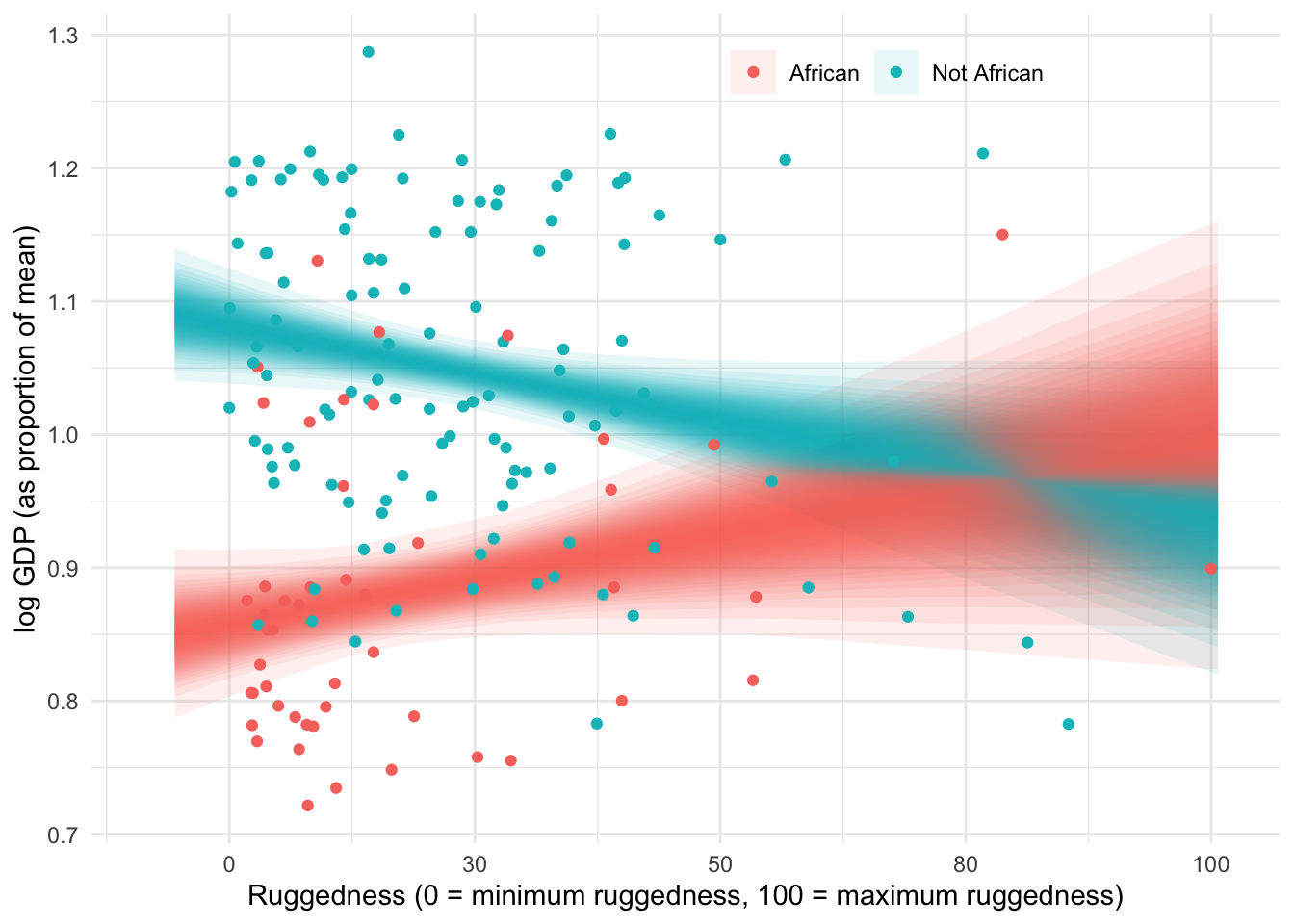
In this vignette we look at the Log gdp per capita of different countries. The more rugged the terrain the lower the gdp is on average, which fits a nice causal story of the harder it is to cross the land the less trade and wealth is created. This story is reversed though when we look at countries in Africa, as seen below in the figure.
What’s to make of the story? Maybe historical slavery has a lasting effect on the economies of african countries, the flatter more accessible regions of africa had slaving?
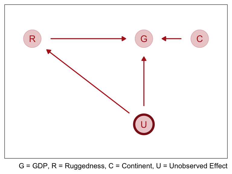
In the graph above we formalize this idea by saying that ruggedness \(R\) influences the current GDP \(G\). Both \(R\) & \(G\) are influenced by some set of unknown confounders \(U\) like proximity to coastline, which we’ll ignore for the moment. Finally \(C\) the continent effects \(G\) as well, crucially \(R\) and \(C\) could be independent or interact on their influence on \(G\). The DAG does not display an interaction, instead we declare outside of the graph like this: \(G = f(R, C)\).
How do we estimate that function \(f\), we could split up the data and make separate models 1 for africa and 1 for all the other continents countries. But this lead to a poor estimate of other parameters like \(\sigma\). Additionally if we wanted to compare models with an information criteria we’d need to use the same data, so splitting the data also hurts that process.
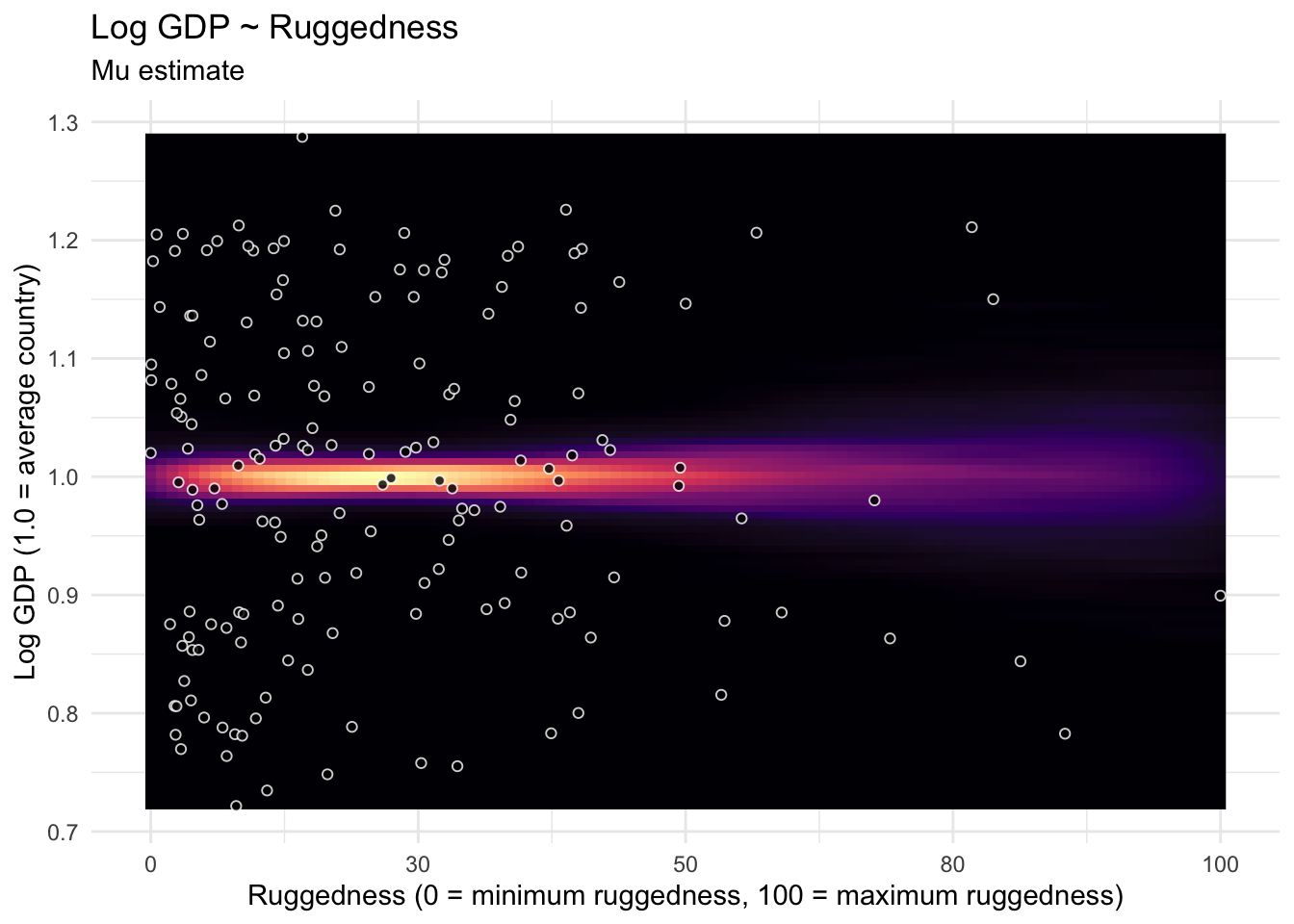
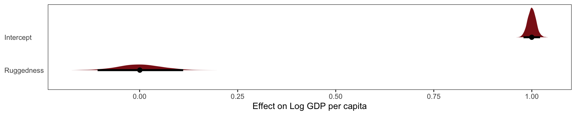
Our first model is:
\[ log(y_i) \ sim Normal(\mu_i, \sigma)\]
\[ \mu_i = \alpha + \beta(\text{rugged}_i - \overline{rugged})\]
Indicator Variable Solution
The first thing to realize is that just including an indicator variable for African nations, won’t reveal the reversed slope.
To build a model that alls nations inside nd outside Africa to have different intercepts, we need to modify the model for \(\mu_i\) so that the mean is conditional on continent. The conventional way to do this would be to just add another term to the linear model:
\[ \mu_i = \alpha + \beta_1(\text{rugged}_i - \overline{rugged}) - \beta_2 \mathbf{I} (\text{Africa}_i)\]
Where \(\text{Africa}_i\) is a 0/1 indicator variable for Africa or not Africa. But this model assumes that african countries have more uncertainty inherently built into their \(mu\) estimate, which makes no sense.
Our simple solution is to create separate intercepts for the different categories, like so:
\[ \mu_i = \alpha_\text{Africa [i]} + \beta_1(\text{rugged}_i - \overline{rugged})\] Where \(\text{Africa [i]}\) is an index variable which takes the value 1 for African nations and 2 for all other nations.
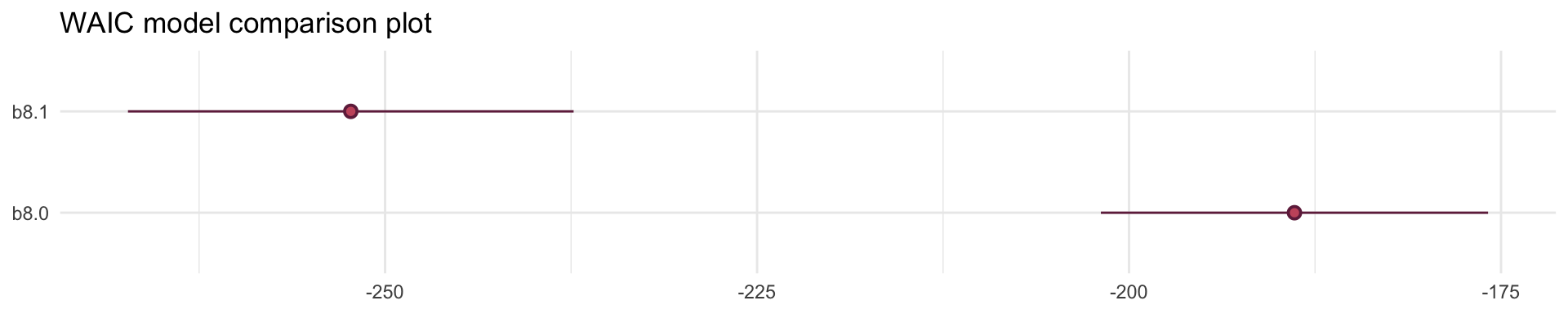
Adding Africa as an index covariate didn’t get that reversal of slopes that we saw in our first plot. But when we compare this model to not having the Africa index covariate with WAIC, its clearly superior. So the Africa variable is clearly picking up some important association in the data. African countries have a lower average Log GDP regardless of their ruggedness and that’s what our African index covariate supports.
     elpd_diff se_diff elpd_loo se_elpd_loo p_loo  se_p_loo looic  se_looic
b8.1    0.0       0.0   126.1      7.5         4.2    0.8   -252.2   15.0
b8.0  -31.7       7.5    94.4      6.5         2.6    0.3   -188.9   13.0
Adding an Interaction does work
How can we we recover the difference in slope that we saw at the beginning of this section? We need a proper interaction effect. This just means we make the slope conditional on whether it’s part of Africa or not.
Just above we modeled
\[ \mu_i = \alpha_\text{Africa [i]} + \beta_1(\text{rugged}_i - \overline{rugged})\]
But now we’re going to make an index for \(\beta\) as well.
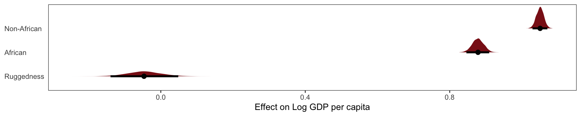
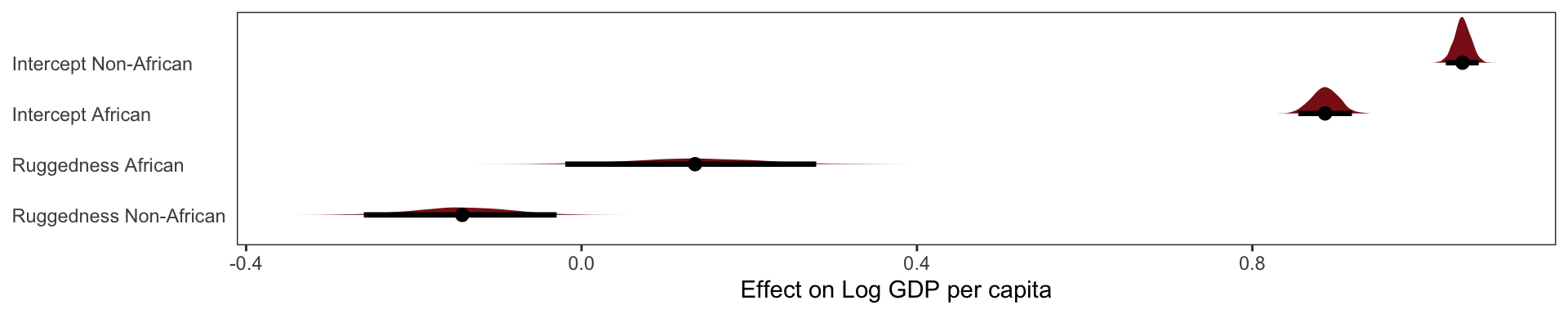
\[ \mu_i = \alpha_\text{Africa [i]} + \beta_\text{Africa[i]}(\text{rugged}_i - \overline{rugged})\]
     elpd_diff se_diff elpd_loo se_elpd_loo p_loo  se_p_loo looic  se_looic
b8.2    0.0       0.0   129.5      7.3         5.0    0.9   -259.1   14.6
b8.1   -3.4       3.3   126.1      7.5         4.2    0.8   -252.2   15.0
b8.0 -35.1 7.5 94.4 6.5 2.6 0.3 -188.9 13.0 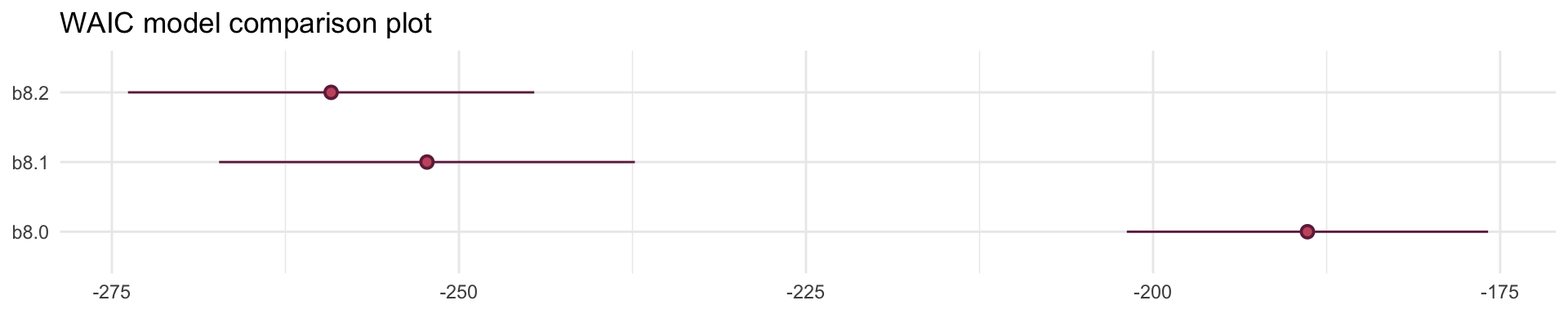
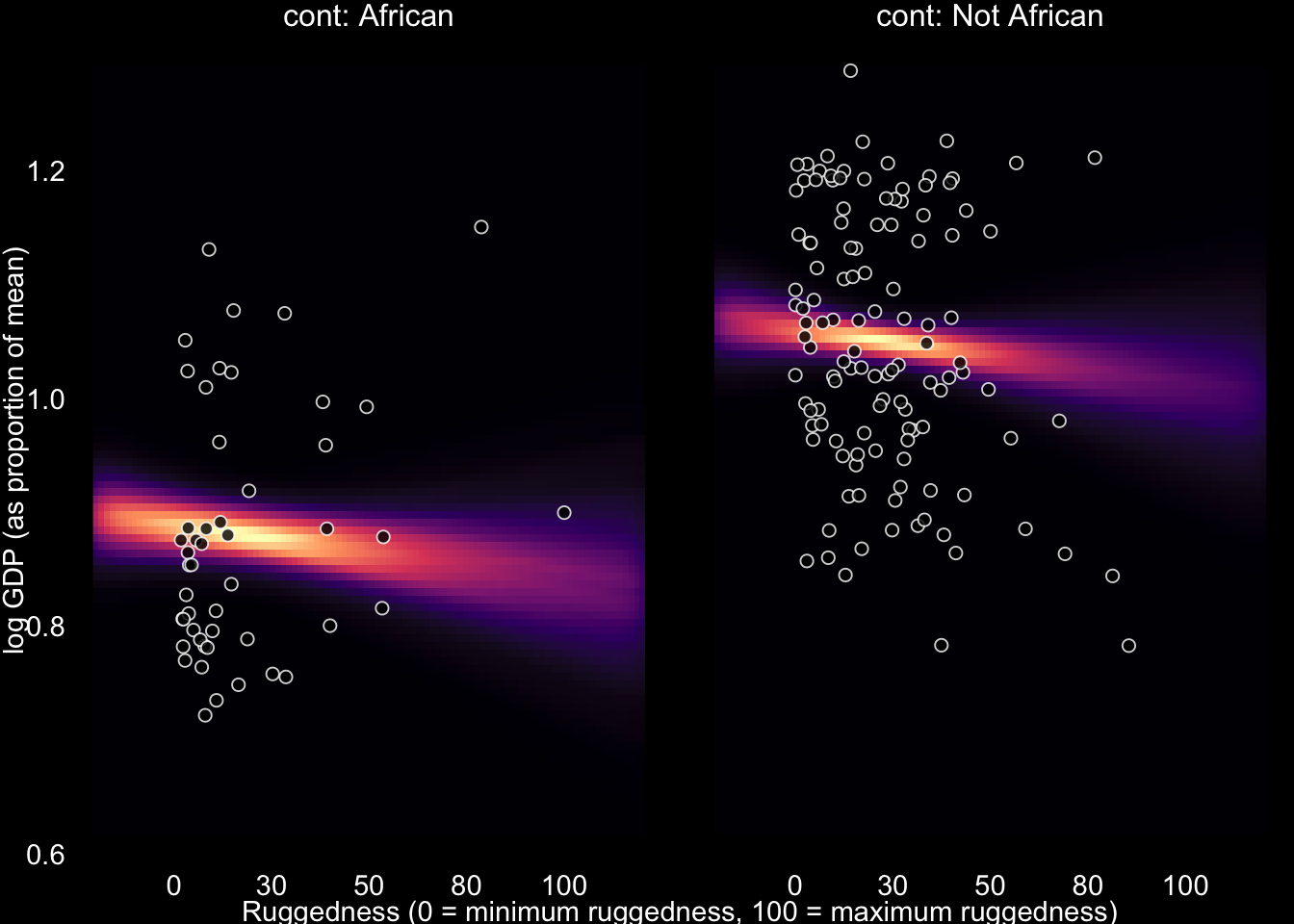
Out interaction model performs best yet, it receives more than 95% of the model weight. Though the remaining weight percentage placed on our 2nd model, does mean there is some reason to think that our model is a bit overfit on its slopes.
The interaction there has two equally valid phrasings. (1) How much does the association between ruggedness and log GDP depend upon whether the nation is in Africa? (2) How much does the association of Africa with log GDP depend upon ruggedness?
While these two possibilities sound different to most humans, our statistical engine thinks they are identical.
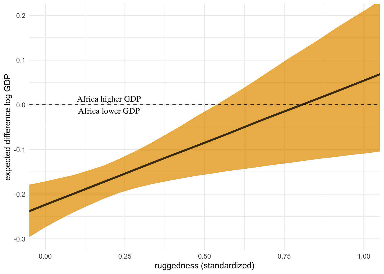
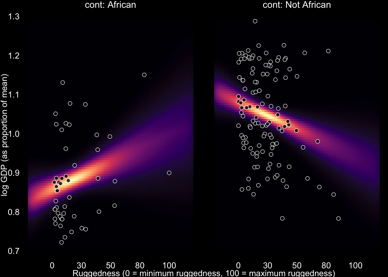
This plot is counter-factual. There is no raw data here. Instead we are seeing through the model’s eyes and imagining comparisons between iden- tical nations inside and outside Africa, as if we could independently manipulate continent and also terrain ruggedness. Below the horizontal dashed line, African nations have lower expected GDP. This is the case for most terrain ruggedness values. But at the highest rugged- ness values, a nation is possibly better off inside Africa than outside it. Really it is hard to find any reliable difference inside and outside Africa, at high ruggedness values. It is only in smooth nations that being in Africa is a liability for the economy.
Simple interactions are symmetric. Within the model, there’s no basis to prefer one interpretation over the other, because in fact they are the same interpretation. But when we reason causally about models, our minds tend to prefer one interpretation over the other, because it’s usually easier to imagine manipulating one of the predictor variables instead of the other. In this case, it’s hard to imagine manipulating which continent a nation is on. But it’s easy to imagine manipulating terrain ruggedness, by flattening hills or blasting tunnels through mountains. Africa’s unusually positive relationship with terrain ruggedness is due to historical causes, not contemporary terrain, then tunnels might improve economies in the present. At the same time, continent is not really a cause of economic activity. Rather there are historical and political factors associated with continents, and we use the continent variable as a proxy for those factors. It is manipulation of those other factors that would matter.
Continuous - Continuous Interactions
Richard McElreath writes:
I want to convince the reader that interaction effects are difficult to interpret. They are nearly impossible to interpret, using only posterior means and standard deviations. Once interactions exist, multiple parameters are always in play at the same time. It is hard enough with the simple, categorical interactions from the terrain ruggedness example. Once we start modeling interactions among more than one continuous variables, it gets much harder. It’s one thing to make a slope conditional upon a category. In such a context, the model reduces to estimating a different slope for each category. But it’s quite a lot harder to understand that a slope varies in a continuous fashion with a continuous variable. Interpretation is much harder in this case, even though the mathematics of the model are essentially the same as in the categorical case.
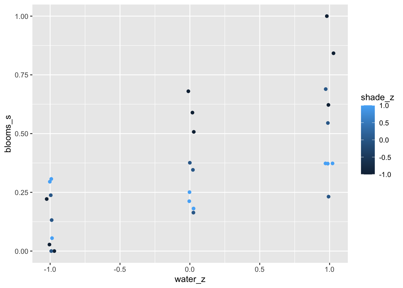
Tulips Example
The data in this example are sizes of blooms from beds of tulips grown in greenhouses, under different soil and light conditions. The blooms column will be our outcome—what we wish to predict. The water and shade columns will be our predictor variables.
Since both light and water help plants grow and produce blooms, it stands to reason that the independent effect of each will be to produce bigger blooms. But we’ll also be interested in the interaction between these two variables. In the absence of light, for example, it’s hard to see how water will help a plant—photosynthesis depends upon both light and water. Like- wise, in the absence of water, sunlight does a plant little good. One way to model such an interdependency is to use an interaction effect. In the absence of a good mechanistic model of the interaction, one that uses a theory about the plant’s physiology to hypothesize the functional relationship between light and water, then a simple linear two-way interaction is a good start. But ultimately it’s not close to the best that we could do.
The causal DAG for this model is quite simple we have \(\text{Water} \rightarrow \text{Bloom} \leftarrow \text{Shade}\). As before the DAG doesn’t tell us the function through which Water and Shade jointly include Bloom. In principle, every unique combination of Water and Shade could have a different mean Bloom. But we’ll start simpler.
Model with No Interaction
\[ \text{Bloom}_i \sim Normal(\mu_\text{Bloom}_i, \sigma)\]
\[ \mu_{\text{Bloom}_i} = \alpha + \beta_W(\text{Water}_i - \overline{Water}) + \beta_S(\text{Shade}_i - \overline{Shade})\]