TLDR

We don’t necessarily care about fitting the data well, we care about making good predictions about the future. Occam’s razor should shape our models so that we prefer parsimonious models all else equal. How do we quantify the “parsimonious-ness” of a model? We have a grab bag of tools to hopefully steer us between the opposing twin dangers of over-fitting or under-fitting.

What are our tools?

(1) Regularizing the prior

• Don’t get to excited about the data

• Same as frequentists use of a penalized likelihood (e.g. Lasso, Ridge)

(2) Scoring Devices

• Information Criteria: AIC BIC, WAIC

• Cross Validation: PSIS-LOO

The Problem with Parameters

Last chapter we spent a lot of time building causal models. Causal models are fantastic because they allow you to see the consequences of changing a variable, i.e. the \(Do(X)\) operation. If we don’t care about understanding the effects of our actions, rather we only want to predict what \(Y\) will be, it’s tempting to put as many variables into our regression as possible. The more variables we add, inevitably our model will fit the data better.

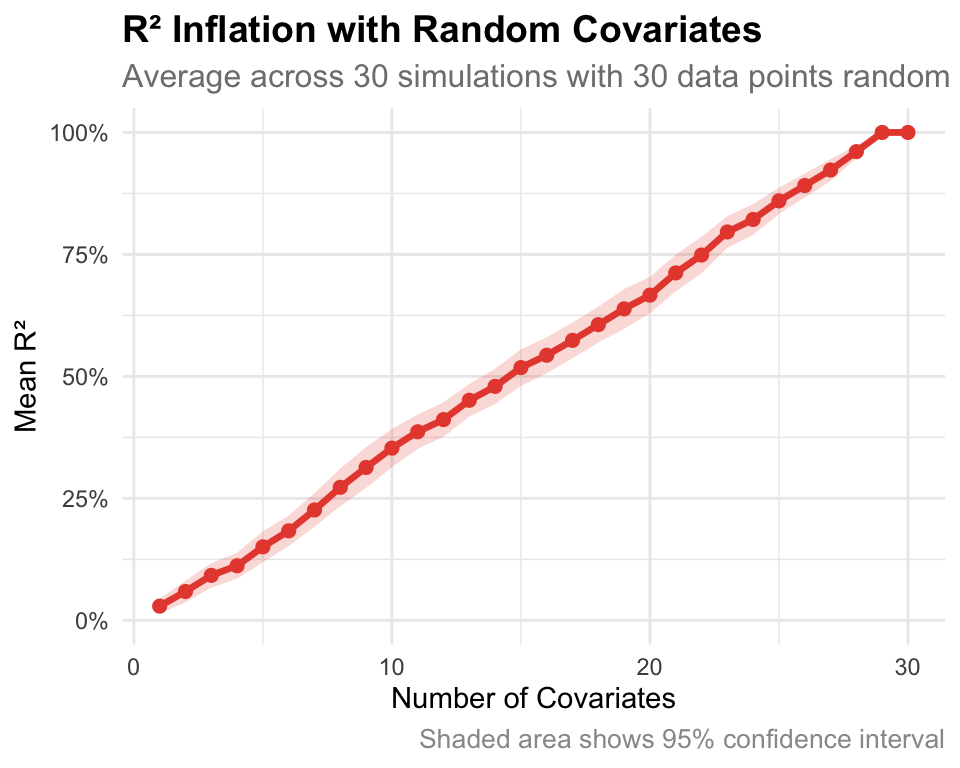
\(R^2\) is a common metric that incentives naive scientists to keep adding variables. \(R^2\) is defined as:

\[R^2 = \frac{\text{var(outcome) - var(residuals)}}{\text{var(outcome)}} = 1 - \frac{\text{var(residuals)}}{\text{var(outcome)}}\]

\(R^2\) always increases as more variables are added even when you just add random numbers which have no relation to the outcome.

While these more complex models predict the data better, they will often predict the new data worse. We have overfitted the data at that point.

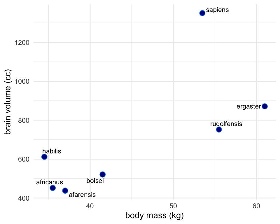
Brain Body Vignette

Plotted below is the relationship between the body size of several primate species and their corresponding brain size. There’s not a strong a priori reason to think body and brain size are perfectly linearly related. The true relationship between brain and body size could be any number of polynomial or log’d functions. Let’s go through a couple to see what’s gained and what’s lost with trying ever more complex functions to fit the data.

Linear

Simplest model is a linear one.

\[\text{Brain Size}_i \sim \text{Normal}(\mu_i, \sigma)\]

\[\mu_i = \alpha + \beta_b\text{Body Mass}_i\]

\[\alpha \sim \text{Normal(0.5, 1)}\]

\[\beta_b \sim \text{Normal(0, 10)}\]

\[\sigma \sim \text{Log-Normal(0, 1)}\]

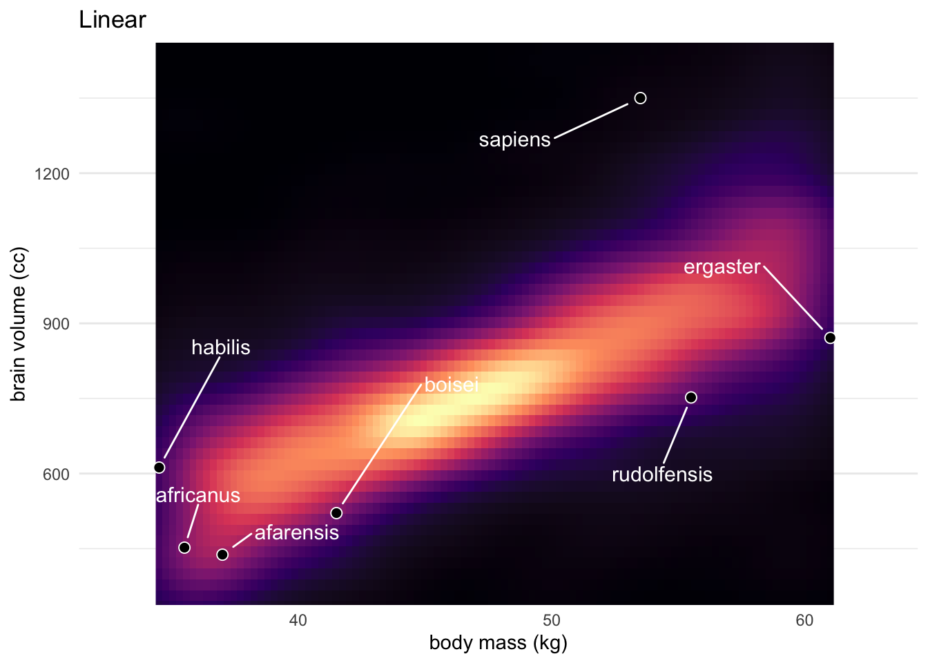
This model has an \(R^2\) value of 0.48

Polynomial

For some comparison models we can add polynomial terms of Mass to our regression. For example the scond degee polynomial that relates body size to brain size is a parabola which has this form:

\[\mu_i = \alpha + \beta_1\text{Body Mass}_i + \beta_2(\text{Body Mass}_i)^2\] We’ll make 4 more models like this each adding another polynomial term like \(\beta_3(\text{Body Mass}_i)^3\), \(\beta_4(\text{Body Mass}_i)^4\)… etc

Below are our six models posterior \(mu\)’s plotted with the data. *Note this is not the posterior predictive distribution since it doesn’t include \(sigma\)

In the figure below I’ve plotted both the heat map for where the model thinks the \(\mu\) estimate should be given all of the data. Additionally I’ve plotted golden lines where I get the best fit lines if I refitted the model by leaving out a different data point each time. This is a “Leave One Out” (LOO) sort of method that helps us see how good our model would do if we didn’t have one of our data points and we wanted to predict it. There are seven of these best fit lines in each model because there are seven different data points we can drop.

For the simple linear 1st order regression we could remove any one point from the sample and get pretty much the same regression line. In contrast, the most complex model 6th order is very sensitive to the sample. The predicted mean would change course a lot, if we removed any one point from the sample. You can see the truth of this in the below plots. On the top left, each line is the best fit for the linear regression. The curves on the bottom right are instead different sixth-order polynomials. Notice that the straight lines hardly vary, while the curves fly about wildly.

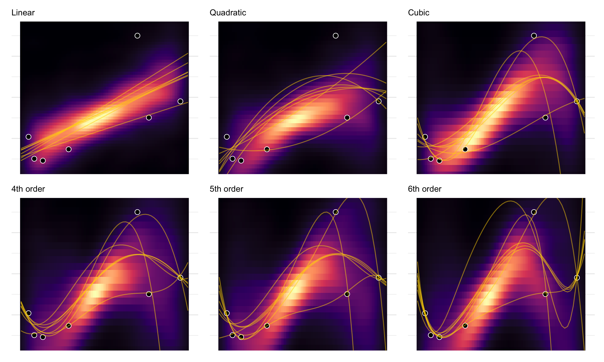
The overfit polynomial models manage to fit the data extremely well, but they suffer for this within-sample accuracy by making nonsensical out-of- sample predictions. In contrast, underfitting produces models that are inaccurate both within and out of sample. They have learned too little, failing to recover regular features of the sample.

Another perspective on the absurd models just above is to consider that model fitting can be considered a form of data compression. Parameters summarize relationships among the data. These summaries compress the data into a simpler form, although with loss of information (“lossy” compression) about the sample. The parameters can then be used to generate new data, effectively decompressing the data.

When a model has a parameter to correspond to each datum, then there is actually no compression. The model just encodes the raw data in a different form, using parameters instead. As a result, we learn nothing about the data from such a model. Learning about the data requires using a simpler model that achieves some compression, but not too much. This view of model selection is often known as Minimum Description Length (MDL).